Classification Intuition#

[2]:

import numpy as np
import pandas as pd

import matplotlib.pyplot as plt
import seaborn as sns
from mpl_toolkits import mplot3d
from graphpkg.static import plot_classification_boundary
import tensorflow as tf
from sklearn.datasets import make_blobs, make_classification, make_regression
import warnings

warnings.filterwarnings("ignore")

Basic Classification#

Target here to generate a data that has only two classes and it can be classified by a linear model also. Like a linear hyperplane can also be a good decision boundary.

[2]:

X, y = make_classification(n_samples=500, n_features=2, random_state=30, \
                           n_informative=1, n_classes=2, n_clusters_per_class=1, \
                           n_repeated=0, n_redundant=0)

print(X.shape, y.shape)

df = pd.DataFrame(X,columns=['x1','x2'])
df['y'] = y

sns.scatterplot(data=df,x='x1',y='x2',hue='y')

(500, 2) (500,)

[2]:

<AxesSubplot:xlabel='x1', ylabel='x2'>

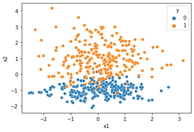
../_images/notebooks_classification_understanding_3_2.png

This is prety much it. linearly classifiable data with 2 classes.

Logistic Regression with Neural network (sigmoid)#

logistic regression is like a linear classification model.

\begin{align} y &= g(h(x))\\ h(x) &= w x + b\\ \text{sigmoid } g(x) &= \frac{1}{1 + e^{-x}} \end{align}

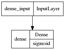
So, actually after a linear weight and bias model, we need a sigmoid. It is actually called a perceptron.

[3]:

model = tf.keras.Sequential([
    tf.keras.layers.Dense(units=1, activation='sigmoid')
])
model.compile(
    optimizer=tf.optimizers.SGD(learning_rate=0.09),
    loss=tf.keras.losses.BinaryCrossentropy(),
    metrics=tf.keras.metrics.BinaryAccuracy()
)

history = model.fit(
    df[['x1','x2']],
    df.y,
    epochs=500,
    batch_size=32,
    verbose=0,
    validation_split = 0.3)

history_metrics = pd.DataFrame(history.history)
history_metrics['epochs'] = history.epoch

[4]:

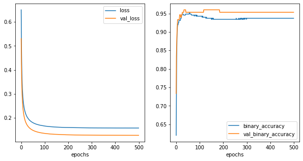
fig,ax = plt.subplots(1,2,figsize=(10,5))
history_metrics.plot(x='epochs',y=['loss','val_loss'],ax=ax[0])
history_metrics.plot(x='epochs',y=['binary_accuracy','val_binary_accuracy'],ax=ax[1])

[4]:

<AxesSubplot:xlabel='epochs'>

../_images/notebooks_classification_understanding_7_1.png

[5]:

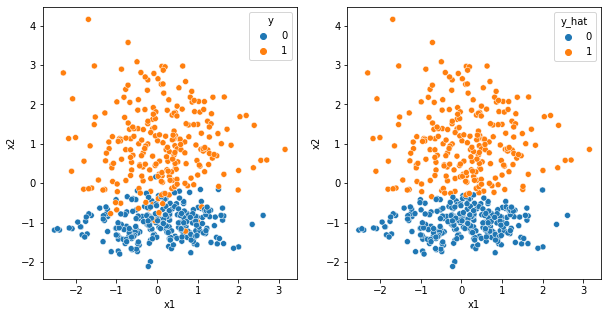
y_hat = model.predict(df[['x1','x2']].values)
df['y_hat'] = np.array(y_hat>0.5,dtype='int')

fig,ax = plt.subplots(1,2,figsize=(10,5))
sns.scatterplot(data=df,x='x1',y='x2',hue='y',ax=ax[0])
sns.scatterplot(data=df,x='x1',y='x2',hue='y_hat', ax=ax[1])

[5]:

<AxesSubplot:xlabel='x1', ylabel='x2'>

../_images/notebooks_classification_understanding_8_1.png

[6]:

tf.keras.utils.plot_model(model,show_layer_activations=True)

[6]:

../_images/notebooks_classification_understanding_9_0.png

[7]:

plot_classification_boundary(model.predict,data=df[['x1','x2','y']].values,size=4,figsize=(7,5))

../_images/notebooks_classification_understanding_10_0.png

Looks to me that it worked out.

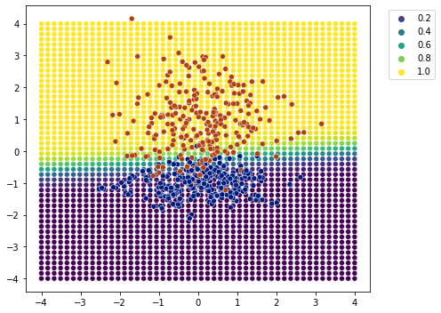
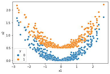
2 sigmoid layers#

[8]:

x1, x2 = make_regression(n_features=1,noise=10, random_state=0, n_samples=500)

x2 = (x2/100)**2

[9]:

df1 = pd.DataFrame()
df1['x1'] = x1[...,-1]
df1['x2'] = x2
df1['y'] = 0

df2 = pd.DataFrame()
df2['x1'] = x1[...,-1]
df2['x2'] = x2 + 0.5
df2['y'] = 1


df = pd.concat((df1,df2)).sample(frac=1)

sns.scatterplot(data=df,x='x1',y='x2',hue='y')

[9]:

<AxesSubplot:xlabel='x1', ylabel='x2'>

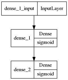
../_images/notebooks_classification_understanding_14_1.png

[10]:

model = tf.keras.Sequential([
    tf.keras.layers.Dense(units=10, activation='sigmoid'),
    tf.keras.layers.Dense(units=1, activation='sigmoid')
])


model.compile(
    optimizer=tf.optimizers.SGD(learning_rate=0.1),
    loss=tf.keras.losses.BinaryCrossentropy(),
    metrics=tf.keras.metrics.BinaryAccuracy()
)

history = model.fit(
    df[['x1','x2']],
    df.y,
    epochs=500,
    batch_size=32,
    verbose=0,
    validation_split = 0.3)

history_metrics = pd.DataFrame(history.history)
history_metrics['epochs'] = history.epoch

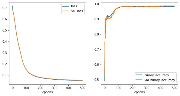
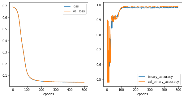
[11]:

fig,ax = plt.subplots(1,2,figsize=(10,5))

history_metrics.plot(x='epochs',y=['loss','val_loss'], ax=ax[0])
history_metrics.plot(x='epochs',y=['binary_accuracy','val_binary_accuracy'], ax=ax[1])

[11]:

<AxesSubplot:xlabel='epochs'>

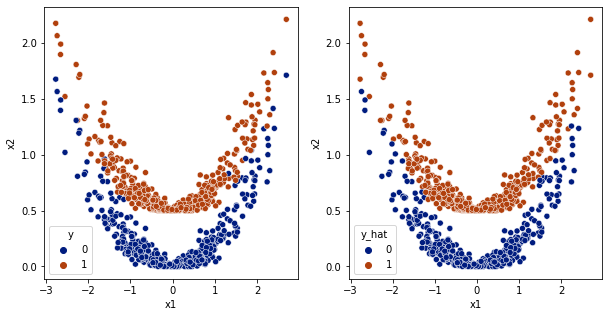
../_images/notebooks_classification_understanding_16_1.png

[12]:

y_hat = model.predict(df[['x1','x2']].values)
df['y_hat'] = np.array(y_hat>0.5,dtype='int')

fig,ax = plt.subplots(1,2,figsize=(10,5))
sns.scatterplot(data=df,x='x1',y='x2',hue='y',ax=ax[0], palette='dark')
sns.scatterplot(data=df,x='x1',y='x2',hue='y_hat', ax=ax[1], palette='dark')

[12]:

<AxesSubplot:xlabel='x1', ylabel='x2'>

../_images/notebooks_classification_understanding_17_1.png

[13]:

tf.keras.utils.plot_model(model,show_layer_activations=True)

[13]:

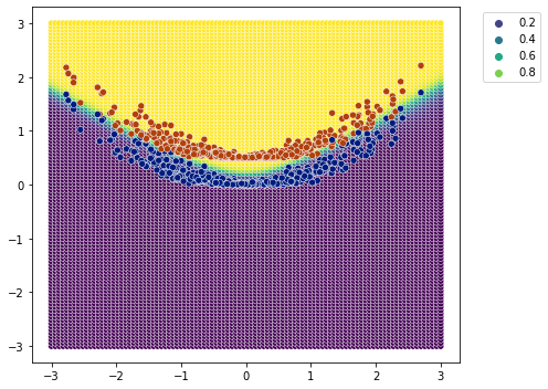
../_images/notebooks_classification_understanding_18_0.png

[14]:

plot_classification_boundary(model.predict,data=df[['x1','x2','y']].values,size=3,\
                            figsize=(7,5), bound_details=100)

../_images/notebooks_classification_understanding_19_0.png

3 sigmoid layers#

[15]:

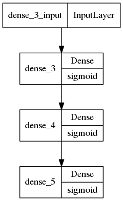
model = tf.keras.Sequential([
    tf.keras.layers.Dense(units=10, activation='sigmoid'),
    tf.keras.layers.Dense(units=10, activation='sigmoid'),
    tf.keras.layers.Dense(units=1, activation='sigmoid')
])


model.compile(
    optimizer=tf.optimizers.SGD(learning_rate=0.1),
    loss=tf.keras.losses.BinaryCrossentropy(),
    metrics=tf.keras.metrics.BinaryAccuracy()
)

history = model.fit(
    df[['x1','x2']],
    df.y,
    epochs=500,
    batch_size=32,
    verbose=0,
    validation_split = 0.3)

history_metrics = pd.DataFrame(history.history)
history_metrics['epochs'] = history.epoch

[16]:

fig,ax = plt.subplots(1,2,figsize=(10,5))
history_metrics.plot(x='epochs',y=['loss','val_loss'], ax=ax[0])
history_metrics.plot(x='epochs',y=['binary_accuracy','val_binary_accuracy'], ax=ax[1])

[16]:

<AxesSubplot:xlabel='epochs'>

../_images/notebooks_classification_understanding_22_1.png

[17]:

y_hat = model.predict(df[['x1','x2']].values)
df['y_hat'] = np.array(y_hat>0.5,dtype='int')

fig,ax = plt.subplots(1,2,figsize=(10,5))
sns.scatterplot(data=df,x='x1',y='x2',hue='y',ax=ax[0], palette='dark')
sns.scatterplot(data=df,x='x1',y='x2',hue='y_hat', ax=ax[1], palette='dark')

[17]:

<AxesSubplot:xlabel='x1', ylabel='x2'>

../_images/notebooks_classification_understanding_23_1.png

[18]:

tf.keras.utils.plot_model(model,show_layer_activations=True)

[18]:

../_images/notebooks_classification_understanding_24_0.png

[19]:

plot_classification_boundary(model.predict,data=df[['x1','x2','y']].values,size=3,\
                            figsize=(7,5), bound_details=100)

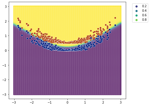
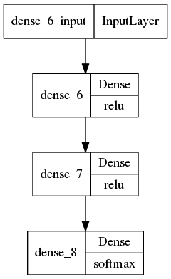
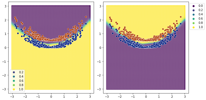
../_images/notebooks_classification_understanding_25_0.png

Something with relu and softmax#

for using softmax i’ll have to one hot encode the target.. so in the final layers we can have two outputs

[20]:

from sklearn.preprocessing import OneHotEncoder

[21]:

ohe = OneHotEncoder()
ohe.fit(df[['y']].values)

y_ohe = ohe.transform(df[['y']].values).toarray()

[22]:

model = tf.keras.Sequential([
    tf.keras.layers.Dense(units=10, activation='relu'),
    tf.keras.layers.Dense(units=10, activation='relu'),
    tf.keras.layers.Dense(units=2, activation='softmax')
])


model.compile(
    optimizer=tf.optimizers.SGD(learning_rate=0.1),
    loss=tf.keras.losses.CategoricalCrossentropy(),
    metrics=tf.keras.metrics.CategoricalAccuracy()
)

history = model.fit(
    df[['x1','x2']],
    y_ohe,
    epochs=500,
    batch_size=32,
    verbose=0,
    validation_split = 0.3
)

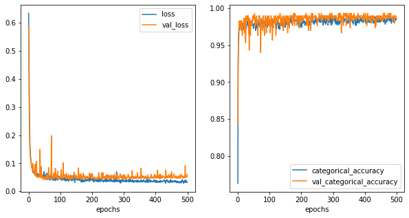
[23]:

history_metrics = pd.DataFrame(history.history)
history_metrics['epochs'] = history.epoch

fig,ax = plt.subplots(1,2,figsize=(10,5))

history_metrics.plot(x='epochs',y=['loss','val_loss'], ax=ax[0])
history_metrics.plot(x='epochs',y=['categorical_accuracy','val_categorical_accuracy'], ax=ax[1])

[23]:

<AxesSubplot:xlabel='epochs'>

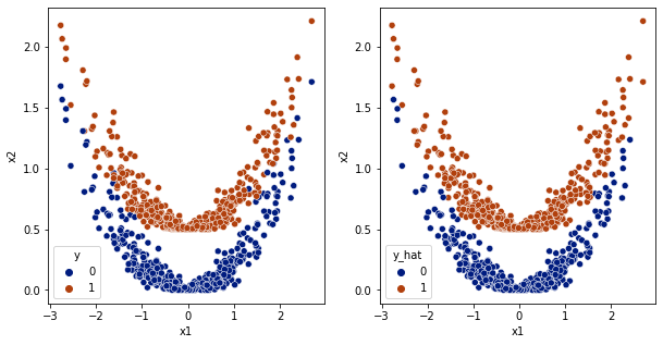
../_images/notebooks_classification_understanding_31_1.png

[24]:

y_hat = np.argmax(model.predict(df[['x1','x2']].values),axis=1)

df['y_hat'] = y_hat

fig,ax = plt.subplots(1,2,figsize=(10,5))
sns.scatterplot(data=df,x='x1',y='x2',hue='y',ax=ax[0], palette='dark')
sns.scatterplot(data=df,x='x1',y='x2',hue='y_hat', ax=ax[1], palette='dark')

[24]:

<AxesSubplot:xlabel='x1', ylabel='x2'>

../_images/notebooks_classification_understanding_32_1.png

[25]:

tf.keras.utils.plot_model(model,show_layer_activations=True)

[25]:

../_images/notebooks_classification_understanding_33_0.png

[26]:

plot_classification_boundary(model.predict,data=df[['x1','x2','y']].values,size=3,\
                            figsize=(10,5), bound_details=100, n_plot_cols=2)

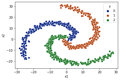
../_images/notebooks_classification_understanding_34_0.png

Easy Spiral Classification#

[27]:

from mightypy.ml.dataset import generate_spiral_data

[28]:

data_limit = 30

X, y = generate_spiral_data(data_limit=data_limit, n_classes=3)

[29]:

df = pd.DataFrame(data=X, columns=['x1','x2'])
df['y'] = y

df = df.sample(frac=1)

sns.scatterplot(data=df, x='x1',y='x2',hue='y',palette='dark')

[29]:

<AxesSubplot:xlabel='x1', ylabel='x2'>

../_images/notebooks_classification_understanding_38_1.png

[30]:

ohe = OneHotEncoder()
ohe.fit(df[['y']].values)

y_ohe = ohe.transform(df[['y']].values).toarray()

1 sigmoid#

[31]:

model = tf.keras.Sequential([
    tf.keras.layers.Dense(units=64, activation='sigmoid'),
    tf.keras.layers.Dense(units=3, activation='softmax')
])


model.compile(
    optimizer=tf.optimizers.SGD(learning_rate=1e-2),
    loss=tf.keras.losses.CategoricalCrossentropy(),
    metrics=tf.keras.metrics.CategoricalAccuracy()
)

history = model.fit(
    df[['x1','x2']],
    y_ohe,
    epochs=500,
    batch_size=32,
    verbose=0,
    validation_split = 0.3
)

history_metrics = pd.DataFrame(history.history)
history_metrics['epochs'] = history.epoch

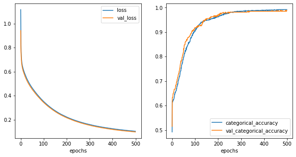
[32]:

fig,ax = plt.subplots(1,2,figsize=(10,5))

history_metrics.plot(x='epochs',y=['loss','val_loss'], ax=ax[0])
history_metrics.plot(x='epochs',y=['categorical_accuracy','val_categorical_accuracy'], ax=ax[1])

[32]:

<AxesSubplot:xlabel='epochs'>

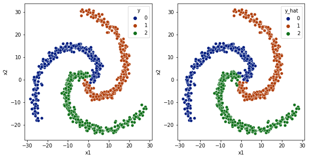
../_images/notebooks_classification_understanding_42_1.png

[33]:

df['y_hat'] = np.argmax(model.predict(df[['x1','x2']].values), axis=1)

fig,ax = plt.subplots(1,2,figsize=(10,5))
sns.scatterplot(data=df,x='x1',y='x2',hue='y',ax=ax[0], palette='dark')
sns.scatterplot(data=df,x='x1',y='x2',hue='y_hat', ax=ax[1], palette='dark')

[33]:

<AxesSubplot:xlabel='x1', ylabel='x2'>

../_images/notebooks_classification_understanding_43_1.png

[34]:

plot_classification_boundary(model.predict,data=df[['x1','x2','y']].values,size=30,\
                            figsize=(15,5), bound_details=100, n_plot_cols=3)

../_images/notebooks_classification_understanding_44_0.png

2 sigmoids#

[35]:

model = tf.keras.Sequential([
    tf.keras.layers.Dense(units=64, activation='sigmoid'),
    tf.keras.layers.Dense(units=64, activation='sigmoid'),
    tf.keras.layers.Dense(units=3, activation='softmax')
])


model.compile(
    optimizer=tf.optimizers.SGD(learning_rate=1e-2),
    loss=tf.keras.losses.CategoricalCrossentropy(),
    metrics=tf.keras.metrics.CategoricalAccuracy()
)

history = model.fit(
    df[['x1','x2']],
    y_ohe,
    epochs=500,
    batch_size=32,
    verbose=0,
    validation_split = 0.3
)

history_metrics = pd.DataFrame(history.history)
history_metrics['epochs'] = history.epoch

[36]:

fig,ax = plt.subplots(1,2,figsize=(10,5))
history_metrics.plot(x='epochs',y=['loss','val_loss'], ax=ax[0])
history_metrics.plot(x='epochs',y=['categorical_accuracy','val_categorical_accuracy'], ax=ax[1])

[36]:

<AxesSubplot:xlabel='epochs'>

../_images/notebooks_classification_understanding_47_1.png

[37]:

df['y_hat'] = np.argmax(model.predict(df[['x1','x2']].values), axis=1)

fig,ax = plt.subplots(1,2,figsize=(10,5))
sns.scatterplot(data=df,x='x1',y='x2',hue='y',ax=ax[0], palette='dark')
sns.scatterplot(data=df,x='x1',y='x2',hue='y_hat', ax=ax[1], palette='dark')

[37]:

<AxesSubplot:xlabel='x1', ylabel='x2'>

../_images/notebooks_classification_understanding_48_1.png

[38]:

plot_classification_boundary(model.predict,data=df[['x1','x2','y']].values,size=30,\
                            figsize=(15,5), bound_details=100, n_plot_cols=3)

../_images/notebooks_classification_understanding_49_0.png

1 relu layer#

[39]:

model = tf.keras.Sequential([
    tf.keras.layers.Dense(units=64, activation='relu'),
    tf.keras.layers.Dense(units=3, activation='softmax')
])


model.compile(
    optimizer=tf.optimizers.Adam(learning_rate=1e-2),
    loss=tf.keras.losses.CategoricalCrossentropy(),
    metrics=tf.keras.metrics.CategoricalAccuracy()
)

history = model.fit(
    df[['x1','x2']],
    y_ohe,
    epochs=500,
    batch_size=32,
    verbose=0,
    validation_split = 0.3
)

history_metrics = pd.DataFrame(history.history)
history_metrics['epochs'] = history.epoch

[40]:

fig,ax = plt.subplots(1,2,figsize=(10,5))
history_metrics.plot(x='epochs',y=['loss','val_loss'], ax=ax[0])
history_metrics.plot(x='epochs',y=['categorical_accuracy','val_categorical_accuracy'], ax=ax[1])

[40]:

<AxesSubplot:xlabel='epochs'>

../_images/notebooks_classification_understanding_52_1.png

[41]:

df['y_hat'] = np.argmax(model.predict(df[['x1','x2']].values), axis=1)

fig,ax = plt.subplots(1,2,figsize=(10,5))
sns.scatterplot(data=df,x='x1',y='x2',hue='y',ax=ax[0], palette='dark')
sns.scatterplot(data=df,x='x1',y='x2',hue='y_hat', ax=ax[1], palette='dark')
plt.show()

../_images/notebooks_classification_understanding_53_0.png

[42]:

plot_classification_boundary(model.predict,data=df[['x1','x2','y']].values,size=30,\
                            figsize=(15,5), bound_details=100, n_plot_cols=3)

../_images/notebooks_classification_understanding_54_0.png

relu as compared to sigmoid, creates sharper edges(more clear probabilities).

2 relu layers#

[43]:

model = tf.keras.Sequential([
    tf.keras.layers.Dense(units=100, activation='relu'),
    tf.keras.layers.Dense(units=100, activation='relu'),
    tf.keras.layers.Dense(units=3, activation='softmax')
])


model.compile(
    optimizer=tf.optimizers.Adam(learning_rate=0.01),
    loss=tf.keras.losses.CategoricalCrossentropy(),
    metrics=tf.keras.metrics.CategoricalAccuracy()
)

history = model.fit(
    df[['x1','x2']],
    y_ohe,
    epochs=500,
    batch_size=32,
    verbose=0,
    validation_split = 0.3
)

history_metrics = pd.DataFrame(history.history)
history_metrics['epochs'] = history.epoch

[44]:

fig,ax = plt.subplots(1,2,figsize=(10,5))
history_metrics.plot(x='epochs',y=['loss','val_loss'], ax=ax[0])
history_metrics.plot(x='epochs',y=['categorical_accuracy','val_categorical_accuracy'], ax=ax[1])

[44]:

<AxesSubplot:xlabel='epochs'>

../_images/notebooks_classification_understanding_58_1.png

[45]:

df['y_hat'] = np.argmax(model.predict(df[['x1','x2']].values), axis=1)

fig,ax = plt.subplots(1,2,figsize=(10,5))
sns.scatterplot(data=df,x='x1',y='x2',hue='y',ax=ax[0], palette='dark')
sns.scatterplot(data=df,x='x1',y='x2',hue='y_hat', ax=ax[1], palette='dark')
plt.show()

../_images/notebooks_classification_understanding_59_0.png

[46]:

plot_classification_boundary(model.predict,data=df[['x1','x2','y']].values,size=30,\
                            figsize=(15,5), bound_details=100, n_plot_cols=3)

../_images/notebooks_classification_understanding_60_0.png

1 layer relu almost did the job. 2 layer relu is almost the same.

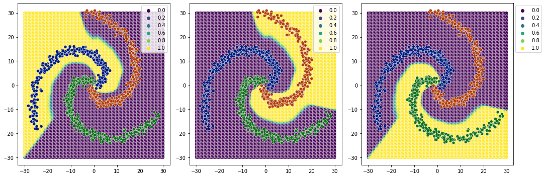
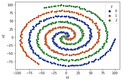
Complex Spiral Classification#

[47]:

data_limit = 100

X, y = generate_spiral_data(data_limit=data_limit, n_classes=3)

df = pd.DataFrame(data=X, columns=['x1','x2'])
df['y'] = y

df = df.sample(frac=1)

sns.scatterplot(data=df, x='x1',y='x2',hue='y',palette='dark')

[47]:

<AxesSubplot:xlabel='x1', ylabel='x2'>

../_images/notebooks_classification_understanding_63_1.png

[48]:

ohe = OneHotEncoder()
ohe.fit(df[['y']].values)

y_ohe = ohe.transform(df[['y']].values).toarray()

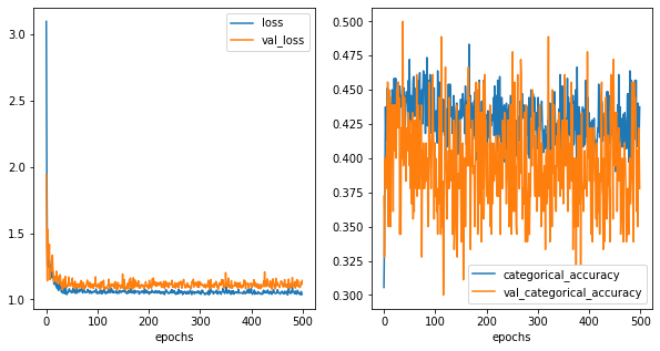
1 relu layer#

[49]:

model = tf.keras.Sequential([
    tf.keras.layers.Dense(units=100, activation='relu'),
    tf.keras.layers.Dense(units=3, activation='softmax')
])


model.compile(
    optimizer=tf.optimizers.Adam(learning_rate=0.01),
    loss=tf.keras.losses.CategoricalCrossentropy(),
    metrics=tf.keras.metrics.CategoricalAccuracy()
)

history = model.fit(
    df[['x1','x2']],
    y_ohe,
    epochs=500,
    batch_size=32,
    verbose=0,
    validation_split = 0.2
)

history_metrics = pd.DataFrame(history.history)
history_metrics['epochs'] = history.epoch

[50]:

fig,ax = plt.subplots(1,2,figsize=(10,5))

history_metrics.plot(x='epochs',y=['loss','val_loss'], ax=ax[0])
history_metrics.plot(x='epochs',y=['categorical_accuracy','val_categorical_accuracy'], ax=ax[1])

[50]:

<AxesSubplot:xlabel='epochs'>

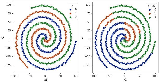
../_images/notebooks_classification_understanding_67_1.png

[51]:

df['y_hat'] = np.argmax(model.predict(df[['x1','x2']].values), axis=1)

fig,ax = plt.subplots(1,2,figsize=(10,5))
sns.scatterplot(data=df,x='x1',y='x2',hue='y',ax=ax[0], palette='dark')
sns.scatterplot(data=df,x='x1',y='x2',hue='y_hat', ax=ax[1], palette='dark')
plt.show()

../_images/notebooks_classification_understanding_68_0.png

[52]:

plot_classification_boundary(model.predict,data=df[['x1','x2','y']].values,size=data_limit,\
                            figsize=(15,5), bound_details=100, n_plot_cols=3)

../_images/notebooks_classification_understanding_69_0.png

So, for 1 relu layer, it is not able to converge. and decision boundaries are not very clear.

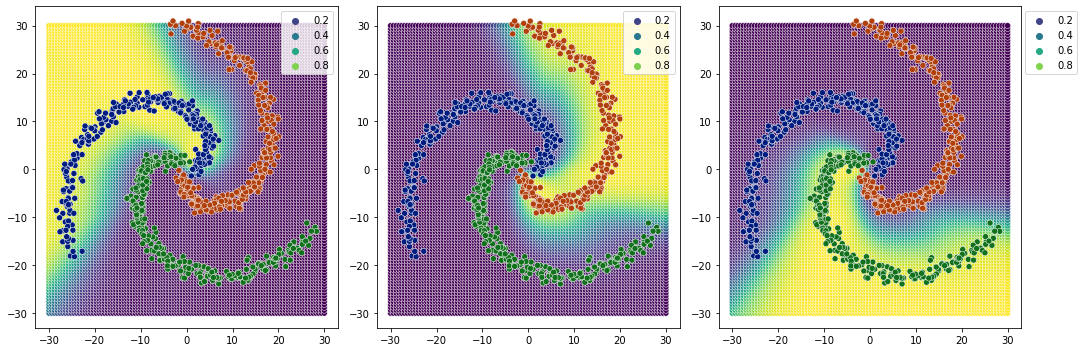
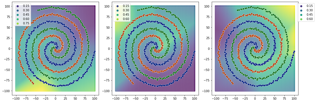
2 relu layers#

[53]:

model = tf.keras.Sequential([
    tf.keras.layers.Dense(units=100, activation='relu'),
    tf.keras.layers.Dense(units=100, activation='relu'),
    tf.keras.layers.Dense(units=3, activation='softmax')
])


model.compile(
    optimizer=tf.optimizers.Adam(learning_rate=0.001),
    loss=tf.keras.losses.CategoricalCrossentropy(),
    metrics=tf.keras.metrics.CategoricalAccuracy()
)

history = model.fit(
    df[['x1','x2']],
    y_ohe,
    epochs=500,
    batch_size=32,
    verbose=0,
    validation_split = 0.3
)

history_metrics = pd.DataFrame(history.history)
history_metrics['epochs'] = history.epoch

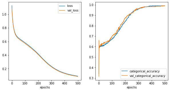
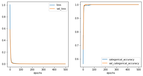
[54]:

fig,ax = plt.subplots(1,2,figsize=(10,5))

history_metrics.plot(x='epochs',y=['loss','val_loss'], ax=ax[0])
history_metrics.plot(x='epochs',y=['categorical_accuracy','val_categorical_accuracy'], ax=ax[1])

[54]:

<AxesSubplot:xlabel='epochs'>

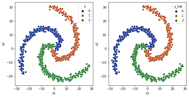
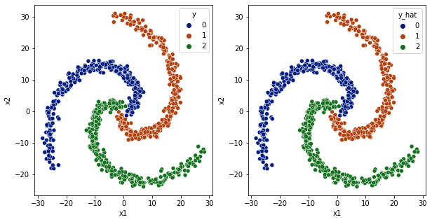
../_images/notebooks_classification_understanding_73_1.png

[55]:

df['y_hat'] = np.argmax(model.predict(df[['x1','x2']].values), axis=1)

fig,ax = plt.subplots(1,2,figsize=(10,5))
sns.scatterplot(data=df,x='x1',y='x2',hue='y',ax=ax[0], palette='dark')
sns.scatterplot(data=df,x='x1',y='x2',hue='y_hat', ax=ax[1], palette='dark')
plt.show()

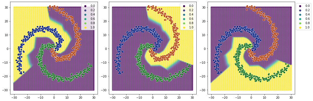
../_images/notebooks_classification_understanding_74_0.png

[56]:

plot_classification_boundary(model.predict,data=df[['x1','x2','y']].values,size=data_limit,\
                            figsize=(15,5), bound_details=100, n_plot_cols=3)

../_images/notebooks_classification_understanding_75_0.png

Clear decision boundaries.

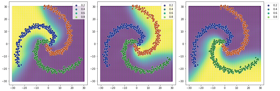
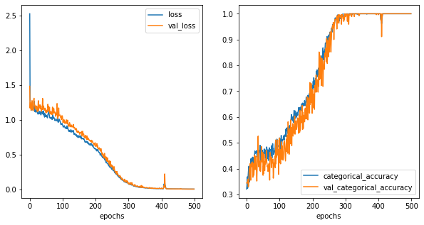
A little bit complex model#

[57]:

model = tf.keras.Sequential([
    tf.keras.layers.Dense(units=100, activation='relu'),
    tf.keras.layers.Dense(units=100, activation='relu'),
    tf.keras.layers.Dense(units=100, activation='relu'),
    tf.keras.layers.Dense(units=100, activation='relu'),
    tf.keras.layers.Dense(units=3, activation='softmax')
])


model.compile(
    optimizer=tf.optimizers.Adam(learning_rate=0.001),
    loss=tf.keras.losses.CategoricalCrossentropy(),
    metrics=tf.keras.metrics.CategoricalAccuracy()
)

history = model.fit(
    df[['x1','x2']],
    y_ohe,
    epochs=500,
    batch_size=32,
    verbose=0,
    validation_split = 0.3
)

history_metrics = pd.DataFrame(history.history)
history_metrics['epochs'] = history.epoch

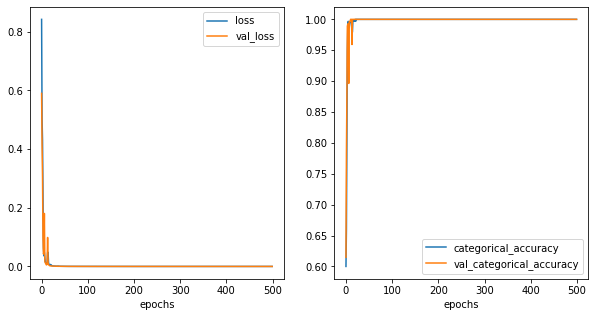
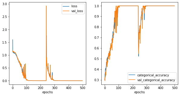
[58]:

fig,ax = plt.subplots(1,2,figsize=(10,5))

history_metrics.plot(x='epochs',y=['loss','val_loss'], ax=ax[0])
history_metrics.plot(x='epochs',y=['categorical_accuracy','val_categorical_accuracy'], ax=ax[1])

[58]:

<AxesSubplot:xlabel='epochs'>

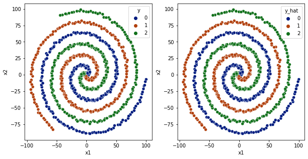
../_images/notebooks_classification_understanding_79_1.png

[59]:

df['y_hat'] = np.argmax(model.predict(df[['x1','x2']].values), axis=1)

fig,ax = plt.subplots(1,2,figsize=(10,5))
sns.scatterplot(data=df,x='x1',y='x2',hue='y',ax=ax[0], palette='dark')
sns.scatterplot(data=df,x='x1',y='x2',hue='y_hat', ax=ax[1], palette='dark')
plt.show()

../_images/notebooks_classification_understanding_80_0.png

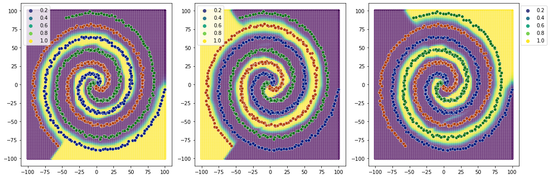
[60]:

plot_classification_boundary(model.predict,data=df[['x1','x2','y']].values,size=data_limit,\
                            figsize=(15,5), bound_details=100, n_plot_cols=3)

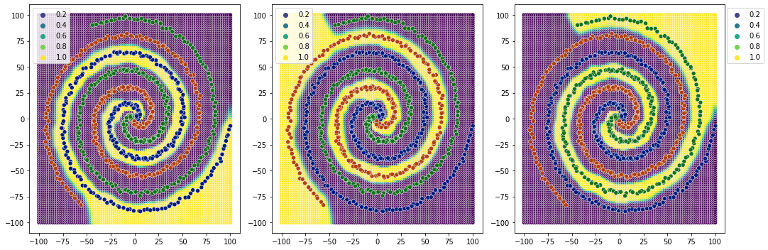
../_images/notebooks_classification_understanding_81_0.png

clearer decision boundaries than 2 relu layers.